When Asset Purchases Actually Increase Long-Term Tax Exposure (and How to Avoid It)
A durable asset purchase plan starts with how deductions and basis changes reappear in the exit-year stack.
High-income Florida taxpayers tend to think about asset purchases in a familiar one-year frame: “Buy it before year-end, get the deduction, reduce the bill.” That mindset can be directionally right—and still produce the wrong lifetime outcome.
In a no–state-income-tax environment, the marginal dollar of federal tax planning carries more weight. The problem is that asset-based deductions are rarely “free”: they usually shift timing, change income character, and reallocate who pays what tax and when. For sophisticated real estate investors and business owners, the long-term exposure often shows up later as:
a higher-tax exit year (depreciation recapture, unrecaptured §1250 gain, NIIT layering),
income stacking that pushes other items into higher tiers,
lost flexibility because the wrong entity/ownership structure locked in the wrong outcome,
or cash-flow strain because deductions were harvested without a plan for the unwind.
This article is a strategic planning guide to asset purchase tax planning—specifically, the scenarios where buying assets (or accelerating depreciation) increases multi-year tax cost, and the planning logic we use to avoid that trap. Our goal is not to talk you into or out of deductions. Our goal is to keep deductions from becoming future tax concentration.
We’ll pressure-test your income stacking across years and identify where depreciation recapture or §1250 exposure could concentrate in an exit year.
Key takeaways
Deductions are not the same as savings. Many “write-offs” are timing shifts that can create a larger, higher-rate tax event later (especially at exit).
Income stacking is the hidden driver. The year you claim deductions and the year you recognize gain matter as much as the asset itself.
NIIT is often the swing factor. The same asset purchase can be neutral or costly depending on whether it expands the 3.8% NIIT base and whether you can structurally reduce that base.
Real estate is an unwind game. Accelerated depreciation (cost segregation, bonus depreciation) is powerful, but it must be paired with an exit/hold strategy and a plan for recapture and unrecaptured §1250 gain.
Entity and ownership structure is not a paperwork decision. It determines character of income, allocation flexibility, passive vs active outcomes, and NIIT exposure.
Cash flow can backfire. A deduction that improves this year’s liquidity can reduce future options if it creates a “tax cliff” later.
A useful way to read the sections that follow: every time you see a proposed asset purchase, run it through the same filter—(1) where does the deduction land in the multi-year stack, (2) what does it do to basis and exit-year character, and (3) does your structure preserve options if facts change.
We’ll map how accelerated depreciation and passive vs active treatment could change your unwind scenario and NIIT layering at disposition.
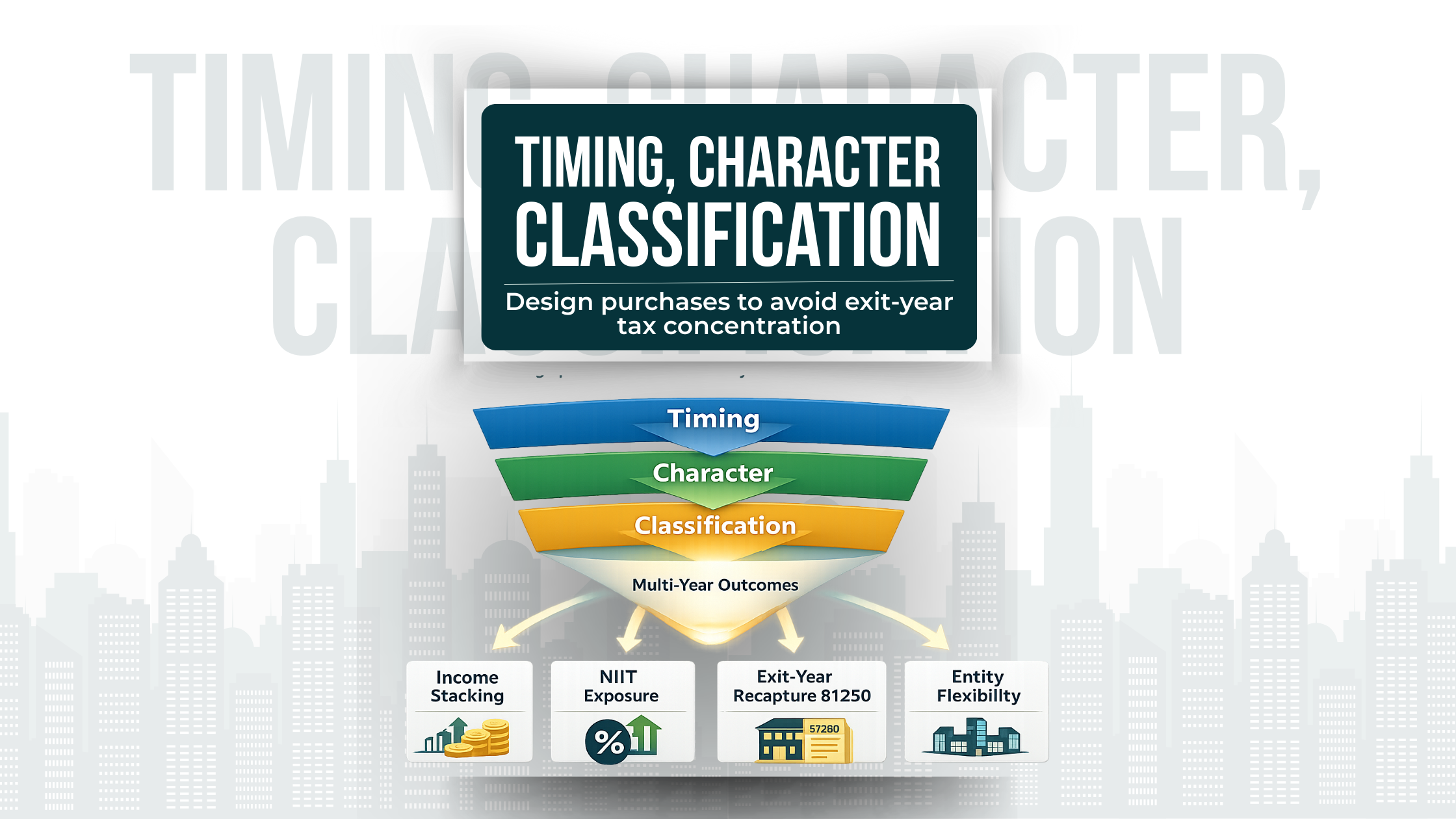
1) The core concept: when an “asset purchase” increases lifetime tax
Asset purchases create tax outcomes through three mechanisms:
Timing (when deductions occur vs when income is recognized)
Character (ordinary income vs long-term capital gain vs special categories like unrecaptured §1250 gain)
Classification (active vs passive; investment vs trade/business; entity-level vs owner-level; NIIT vs non-NIIT base)
The long-term exposure arises when a purchase strategy optimizes only timing (this year), while inadvertently worsening character/classification later.
A diagnostic we use with sophisticated taxpayers:
If the deduction is harvested in a year where your marginal rate is “low” for you (or the loss is not usable), and the basis reduction pushes more income into a later year where your stack is already high, the move often raises lifetime tax.
If the purchase shifts future income into categories taxed at higher effective rates (ordinary recapture, NIIT-included base), the move often raises lifetime tax.
If the purchase locks you into an ownership/structure path that reduces flexibility at exit (allocation constraints, passive loss traps, double-tax considerations), the move often raises lifetime tax.
This is not an argument against depreciation. It’s a design argument: depreciation is a tool. Tools require a plan.
Two contexts where this shows up most:
Real estate acquisitions and renovations. You control depreciation cadence (standard, cost segregation, bonus where applicable) and you later control disposition cadence (sell, refinance, exchange, gift, partial disposition). The unwind is in the same ecosystem as the deduction.
Business acquisitions structured as asset deals (or deemed asset deals). Purchase price allocation and entity choice determine the buyer’s future depreciation/amortization profile—but also determine how much of future proceeds will be ordinary vs capital upon a later sale, and how much future cash flow is effectively “prepaid” through amortization of intangibles. The acquisition model you choose today becomes the tax character you live with at exit.
A subtle but important second-order effect in business asset acquisitions: an allocation that maximizes near-term amortization/depreciation can also increase the portion of a later sale that is treated as ordinary income (for “ordinary” assets and recapture) rather than long-term capital gain. That can be a good trade if your exit-year stack is designed for it—and a costly trade if it lands in an already high ordinary-income year.
2) Income stacking: why the sequence of years drives outcomes
For high earners, the incremental tax rate on the “next dollar” is rarely just the federal bracket. It’s an effective marginal rate that layers:
ordinary brackets,
long-term capital gain brackets,
NIIT once you cross statutory thresholds,
and the character mix of the year (W-2/SE income, K-1 income, rental income, portfolio income, gain events).
For 2026 ordinary income brackets, the IRS inflation-adjusted tables show the bracket breakpoints by filing status.
2026 ordinary income tax brackets (taxable income)
| Filing status | 10% | 12% | 22% | 24% | 32% | 35% | 37% |
|---|---|---|---|---|---|---|---|
| Single | $0–$12,400 | $12,401–$50,400 | $50,401–$105,700 | $105,701–$201,775 | $201,776–$256,225 | $256,226–$640,600 | $640,601+ |
| Married filing jointly | $0–$24,800 | $24,801–$100,800 | $100,801–$211,400 | $211,401–$403,550 | $403,551–$512,450 | $512,451–$768,700 | $768,701+ |
| Married filing separately | $0–$12,400 | $12,401–$50,400 | $50,401–$105,700 | $105,701–$201,775 | $201,776–$256,225 | $256,226–$384,350 | $384,351+ |
| Head of household | $0–$17,700 | $17,701–$67,450 | $67,451–$105,700 | $105,701–$201,750 | $201,751–$256,200 | $256,201–$640,600 | $640,601+ |
Why this matters for asset purchases: accelerated depreciation is most valuable when it offsets income that would otherwise sit in your highest marginal layers. But if you pull deductions forward into a year where you’re already at a lower marginal layer (or can’t use the losses due to passive rules), you may be trading away flexibility and creating a higher-tax unwind later.
There is a second-order effect high-income taxpayers often miss: even if the deduction reduces taxable income, it can change what else becomes “marginal.” For example, it can shift how much of your long-term gain is taxed at each bracket tier, how much NIIT is triggered, and which items become the “top layer” of income that determines the effective rate on the next dollar.
The “three-year stacking” example (conceptual)
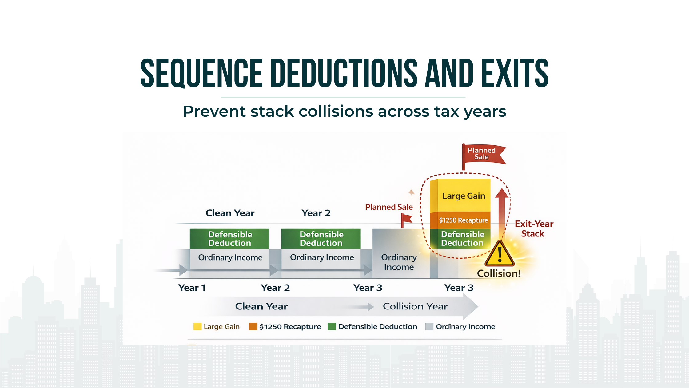
Sequencing is about placing deductions in expensive years while keeping exit years structurally clean.
Year 1: You have unusually high ordinary income (business surge, large bonus, major deal close).
Year 2: Income normalizes.
Year 3: You plan a property sale or business sale event.
If you accelerate depreciation in Year 2 because it “feels like the right time,” you may be missing the true opportunity (Year 1 high-rate offset) and increasing the Year 3 tax exposure if the depreciation reduces basis and increases the §1250 stack.
A more sophisticated approach is to treat deductions as a resource you “spend” where they buy the most marginal-rate relief, while building a sale-year glidepath that avoids compressing multiple high-character items into one year. Practically, that often means:
selecting which assets become deduction engines and which assets remain clean exit assets,
staging renovations and placed-in-service dates across years rather than clustering,
and sequencing dispositions so the year of largest gain is not also the year of largest ordinary income.
A common failure mode is the exit-year pileup: multiple properties (or a business plus property) sold in the same year because it is operationally convenient. In that case, deductions taken years earlier can backfire by increasing the portion of gain taxed at higher effective layers in the pileup year.
One more sequencing nuance that matters for sophisticated investors: deduction timing can change your negotiating posture. If you have accelerated amortization/depreciation from a business asset acquisition, you may feel pressured to exit sooner to “harvest value,” even when the optimal tax year to exit is later. A coordinated plan treats the exit year as a controlled variable whenever economics allow—and avoids letting last year’s deduction strategy force this year’s sale decision.
3) NIIT: the surtax that quietly flips the decision
The Net Investment Income Tax applies at 3.8% on the lesser of net investment income or the excess of modified adjusted gross income over statutory thresholds. That 3.8% is not a rounding error at scale; it is a persistent layer that turns “close” decisions into clear decisions.
Why NIIT changes asset purchase tax planning:
Real estate income that is treated as investment (or passive rental without material participation) may sit in NIIT base.
A sale year with capital gains can push you over the threshold and expose more income to NIIT.
A “deduction-heavy” year may reduce MAGI enough to avoid NIIT—but if the deduction is mostly timing and the unwind happens in a high-gain year, NIIT can return with force.
The advanced planning question is not “How do we avoid NIIT?” It is:
Which parts of our income stack are structurally NIIT-included, which parts are not, and what events turn a low-NIIT year into a high-NIIT year?
Two levers matter most in practice:
1) Classification and participation discipline. For real estate investors, NIIT exposure often hinges on whether income is treated as from a trade or business in which you materially participate versus passive/investment income. In mixed portfolios (STR operations, long-term rentals, partnerships), classification is not just a tax return outcome; it’s a facts-and-records outcome. When classification is loose, the exit-year NIIT surprise is common.
2) Timing the trigger year. Even when NIIT applies, you can often reduce its impact by controlling the year you cross the threshold. Asset purchases that lower MAGI in a year that would have been a high-gain year can be valuable. The same purchases in a year that wasn’t going to trigger NIIT anyway can be wasted, especially if they increase basis reduction and drive a larger gain into a future year that will trigger NIIT.
A third lever is often overlooked by sophisticated taxpayers who have multiple advisors: entity and ownership alignment. The NIIT base is not only about what you own, but how you own it—direct, through partnerships, through trusts, or through structures where income character and participation do not align with the economic reality. If your structure forces investment characterization, asset purchase deductions that increase future gain can also increase future NIIT base.
Finally, NIIT interacts with multi-year planning in a way that punishes fragmentation: you can “win” on NIIT in a deduction year and “lose” more than you saved in the disposition year. The remedy is not to stop using deductions. The remedy is to treat NIIT as part of the unwind model whenever a plan reduces basis or accelerates amortization.
4) Real estate exit mechanics: depreciation recapture and unrecaptured §1250 gain
Real estate is where asset purchases most commonly increase long-term exposure—because the unwind is structured:
Depreciation reduces basis.
Lower basis increases gain on sale.
Portions of that gain are taxed differently depending on depreciation history and asset type.
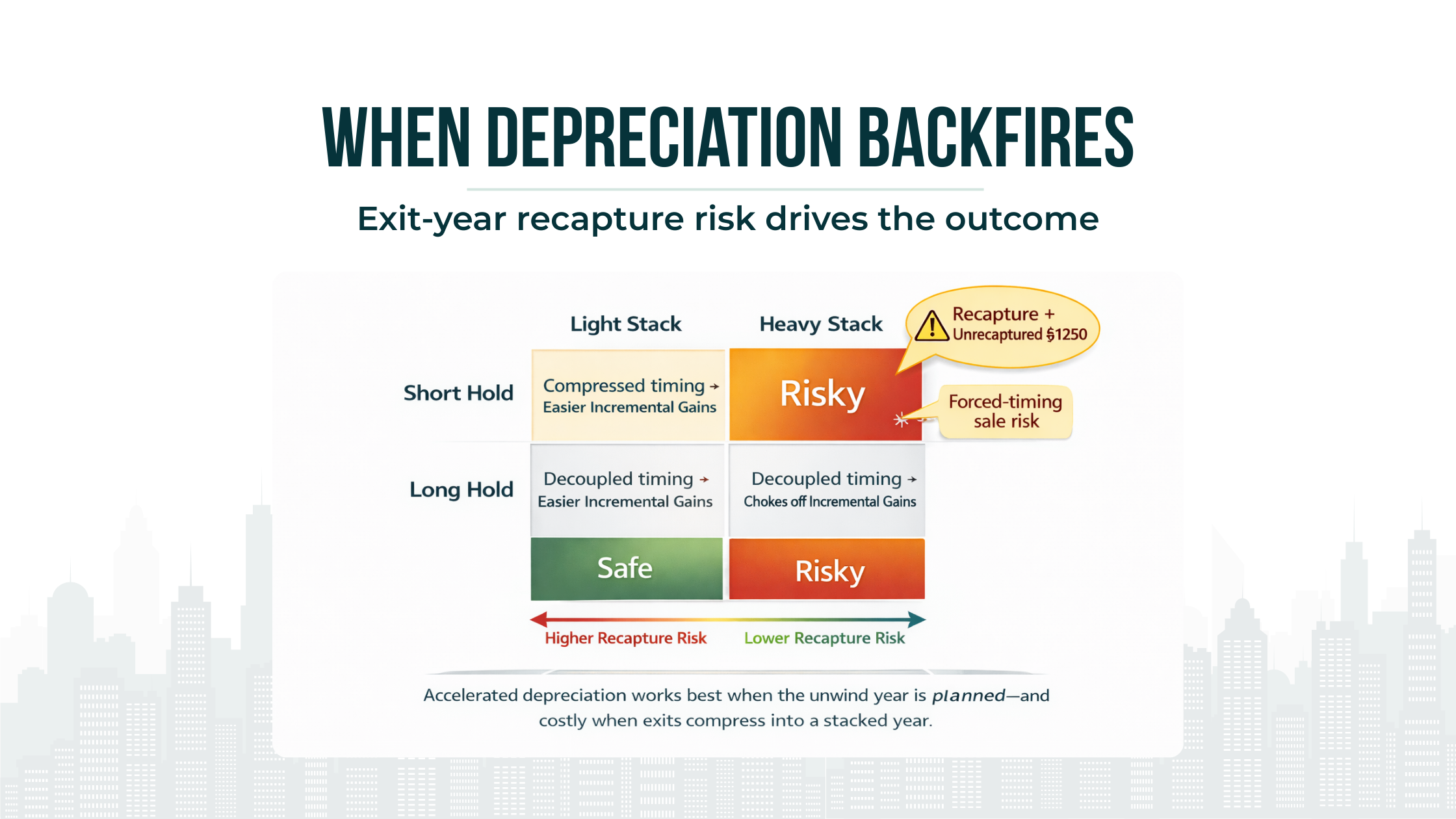
Accelerated depreciation works best when the unwind year is planned—and costly when exits compress into a stacked year.
A key category is unrecaptured §1250 gain: the portion of gain from selling §1250 real property attributable to depreciation, subject to a maximum 25% rate. Even without leaning on the precise rate in your internal modeling, the strategic point is the same:
Accelerated depreciation converts part of your future appreciation into a higher-tax stack at exit.
Where sophisticated investors get surprised is not the existence of recapture—it is the composition of recapture after “smart” depreciation planning.
Cost segregation changes the character mix. When you shift components into shorter-lived property, you typically shift more depreciation into categories that can be recaptured at ordinary income rates when sold (for §1245 components) rather than the unrecaptured §1250 bucket. That can be a good trade in a high ordinary-income year if you hold long enough and reinvest the tax deferral at attractive returns. It can be a bad trade if you sell sooner than expected, or if the sale year is already stacked with ordinary income.
The timing of improvements matters as much as the acquisition. Florida portfolios often have frequent improvement cycles (hurricane hardening, insurance-driven upgrades, STR refreshes). Each placed-in-service decision changes basis and future character. If you consistently front-load depreciation on improvements without a sale-year framework, you can create a property that looks “efficient” on annual returns but produces an expensive unwind when you exit.
A second-order effect worth planning: recapture can interact with the rest of your income stack in ways that change what is marginal. In an exit year that already includes business income, portfolio income, and perhaps a second disposition, the recapture layers can become the “top layer” that pushes other items (including capital gains) into higher effective tiers and increases NIIT exposure. The combined effect is not linear; it’s stack-sensitive.
Another unwind scenario we plan for explicitly is the “forced timing” sale: a sale triggered by insurance renewal failure, casualty-driven capex, partner conflict, or liquidity needs. Forced sales are the reason “we’ll just hold longer” is not a complete plan. If a meaningful portion of your portfolio has non-trivial forced-sale probability, you need to be more conservative about accelerating depreciation that enlarges the ordinary/recapture stack in any near-term exit year.
5) Cost segregation (and bonus depreciation): tools, not tactics
Cost segregation is often treated as a tactic: “run a study, create losses.” In sophisticated planning, it is a capital allocation decision:
It changes the depreciation schedule (timing).
It changes the character and composition of gain on sale (unwind).
It affects suspended losses, especially for passive investors.
It interacts with refinancing, hold periods, and sale sequencing.
Where it increases long-term tax exposure:
short hold periods or high probability of sale during a peak-income year,
portfolio behavior where multiple sales cluster into one year (“exit-year pileup”),
investor profile where losses are not currently usable (passive limitations), making the upfront “benefit” more illusion than savings,
no plan for forced-sale scenarios (insurance/casualty, tenant concentration, or capital needs).
Where it often works best:
long-hold assets with stable cash flow where the time value of money and reinvestment capacity are meaningful,
scenarios where accelerated deductions offset income that is truly expensive (high marginal layers) and are reinvested into high-return opportunities,
portfolios with deliberate sequencing: deductions harvested when income is highest; exits managed when income is lower—or structured so the unwind is controlled.
A refinement many high earners miss: cost segregation should be paired with a disposition menu, not just a hold assumption. Your future options are typically some combination of (a) sell, (b) refinance and hold, (c) exchange into a new asset, (d) partial sale/partner buyout, (e) gift/estate planning transfer, or (f) convert use. Each option treats depreciation history differently. If you have a high probability of selling into a compressed timeline, the cost segregation decision should be made with that probability-weighted exit in mind.
Finally, remember that cost segregation is not only about taxes. It can influence real-world choices: aggressive front-loaded deductions can create psychological permission to overpay for an asset (“the write-off makes it fine”), under-reserve for volatility, or accept weaker operating fundamentals. When that happens, the tax plan becomes part of the reason you are forced to exit early—right when the unwind is least favorable.
6) Asset-based planning vs “deduction-first” planning
A deduction-first plan starts with: “What can we buy?”
An asset-based plan starts with: “What is the investor’s base case over 3–10 years?”
Asset-based planning asks:
What is the likely hold period?
How likely is a sale driven by non-tax factors (insurance changes, casualty risk, tenant concentration, capital needs)?
What is the probability the sale year is also a high-income year?
Will the investor do exchanges, gifts, charitable transfers, or estate transfers?
Which entity structure preserves flexibility if facts change?
Then—and only then—does it select depreciation tools.
The same logic applies in business acquisitions. If you are buying a business (or buying a major set of assets), the deduction-first instinct often becomes: “Allocate as much as possible to fast depreciation and amortization.” That may help near-term after-tax cash flow. It can also increase long-term tax exposure if it creates (a) a larger ordinary-income component on a later sale of those assets, (b) mismatched allocations that constrain negotiations or invite post-closing friction, or (c) a structure that makes the eventual exit a higher-cost event.
Asset-based planning treats the acquisition as one phase of a longer lifecycle: buy, operate, improve, distribute, and eventually exit. Each phase has a different “optimal” mix of timing and character—and the plan coordinates them rather than optimizing only the buy phase.
7) Entity and ownership structure: how gains flow, allocate, and get taxed
The same asset purchase can be tax-efficient or tax-expensive depending on where it sits:
Individual ownership vs partnership vs S corporation vs C corporation (and how debt, distributions, and allocations function).
Who participates (active vs passive), and whether that participation is documented and consistent.
How income and gain are allocated among owners (including special allocations where appropriate and supportable).
Whether the structure preserves optionality for an exit (sale of assets vs sale of equity, partial sales, redemptions, installment considerations).
Why structure affects long-term exposure:
It can shift income into categories more exposed to NIIT or less eligible for certain offsets.
It can trap depreciation and losses where they are less usable.
It can limit flexibility to separate operating risk from property ownership—important in Florida where insurance/casualty risk is not theoretical.
Two structure-driven failure modes show up repeatedly with high-income taxpayers:
1) “Wrong entity for the exit you actually want.” In business acquisitions, buyers often prefer asset deals for basis step-up and depreciation, while sellers often prefer equity deals for rate/character reasons. If you acquire or hold in a structure that forces an asset sale later (or forces a corporate-level tax layer), you may be locking in a more expensive exit than your economics require. A sophisticated plan anticipates the likely buyer profile and the likely sale form and chooses structure with that endpoint in mind.
2) “Ownership misalignment that reduces flexibility.” Multi-owner real estate and operating businesses evolve: new partners, partial redemptions, changes in participation, changes in property use. If the ownership structure cannot adapt (or if it creates uneven exposure to recapture), you can end up selling earlier, selling differently, or selling in a worse year simply to resolve internal constraints. That is a tax cost created by structure, not by markets.
In advanced asset purchase tax planning, we treat entity design as a lever for optionality. Optionality is not abstract: it is the ability to choose when you recognize gain, how you recognize it, and who bears which character of that gain.
A deal-structure note that frequently matters in business asset purchases: purchase price allocation is not just a “tax form” exercise. Allocation decisions affect future amortization/depreciation and can also shape the character of income on an eventual resale. When entity choice and allocation strategy are made independently, investors often get “good” deductions now and a less favorable exit profile later.
8) Active vs passive treatment: where this becomes binding at exit
Passive activity rules are not just a current-year issue. They determine:
whether losses from accelerated depreciation are currently usable,
whether losses are suspended and released only on disposition,
and how much of your “tax benefit” is simply deferred—not saved.
The exit-year interaction is critical:
If you’ve accumulated suspended passive losses, a disposition can release them—but they may offset income in a year that is already dominated by capital gain and §1250 stacking.
If you planned on those losses to reduce tax on ordinary income, but the release happens in a year where the marginal effect is weaker, your strategy underperforms.
Sophisticated planning ties participation, portfolio design, and sale sequencing together:
Which assets are likely to sell sooner?
Which assets should be “deduction engines”?
Which assets should be “clean exit” assets with less depreciation complexity?
A nuance that matters for higher earners with mixed activity types: passive vs non-passive classification is often not stable across time. STR activity can become more operational; long-term rentals can become more passive; partnership roles change. When classification changes, your past depreciation profile does not change—but the way losses can be used (and whether income is NIIT-included) can. That’s why the planning has to be lifecycle-based, not tax-return-year based.
9) Capital gains brackets: why “0/15/20” is not the whole story
For 2026, the IRS inflation-adjusted guidance provides the thresholds for the long-term capital gains 0% and 15% maximum rate amounts by filing status.
2026 long-term capital gain thresholds (taxable income)
| Filing status | 0% up to | 15% up to | 20% above |
|---|---|---|---|
| Married filing jointly / surviving spouse | $98,900 | $613,700 | $613,700+ |
| Married filing separately | $49,450 | $306,850 | $306,850+ |
| Head of household | $66,200 | $579,600 | $579,600+ |
| Single (all other individuals) | $49,450 | $545,500 | $545,500+ |
Why asset purchases still matter even when you “expect” capital gain rates:
Real estate dispositions are rarely pure long-term capital gain. The gain stack commonly includes:
ordinary income recapture components,
unrecaptured §1250 gain (separate cap),
long-term capital gain,
plus potential NIIT layering.
So the relevant planning question becomes:
What is the composition of the exit-year stack, and how does this asset purchase change it?
A related nuance: in business asset contexts, “capital gain” is often a blended outcome across asset classes. Inventory, receivables, and certain intangibles can produce ordinary income treatment. Depreciable equipment can generate ordinary recapture. Goodwill and certain intangibles can behave differently depending on facts and allocations. When you allocate purchase price aggressively to maximize immediate deductions, you may be increasing the ordinary-income portion of gain on a later sale—effectively trading future capital gain for future ordinary income.
Even in pure real estate scenarios, capital gain bracket framing can be misleading because it ignores the role of stack management. Your real planning target is not a rate in isolation—it’s the composition and ordering of the year’s income layers, including how much of the year becomes NIIT-included and how much becomes recapture-driven.
10) Cash flow vs long-term tax efficiency: where strategies backfire
Asset purchases are often justified by liquidity: “We’ll reduce tax now and keep cash.”
That can be rational—unless the strategy creates a future constraint that is more expensive than the cash saved. Backfire patterns we see:
deduction-driven capex that increases maintenance burden and insurance exposure without improving long-term asset quality,
front-loading depreciation and then needing to sell earlier than planned due to market/insurance/casualty realities—turning “savings” into a higher-tax exit,
overleveraging because “paper losses” made the investor feel safer than they were; then a downturn forces dispositions at the worst possible income-stacking moment,
ignoring reserves in a climate- and insurance-sensitive market; the tax plan assumes stability, but the real world forces liquidity events.
A second-order effect for high earners: liquidity-driven deductions can distort deal selection. If an investor is choosing between two assets and the “deduction profile” becomes a deciding factor, there is a risk the tax tail is wagging the investment dog. A high-quality investment often outperforms a tax-optimized mediocre investment even after taxes. Asset purchase tax planning should improve outcomes for good deals, not justify weak ones.
Practically, we like to separate two decisions:
Investment decision: does the asset stand on its own economics?
Tax decision: given the asset, what depreciation cadence preserves flexibility and minimizes lifetime tax?
When those decisions are blended, the backfire rate increases.
11) Retirement, pensions, and RMD coordination: why purchases can raise future exposure
Many high-income Florida taxpayers are in a transition arc:
peak earning years now,
higher mandatory income later (RMDs, pension streams),
and often large embedded gains in real estate and businesses.
Asset purchase decisions should be coordinated with that arc:
Accelerating deductions in years where income will later be structurally high may be valuable—but only if the future unwind years are also planned.
If future RMD years are likely to be high ordinary-income years anyway, pushing more gain into those years can be costly.
Conversely, if you can intentionally create lower-income windows (pre-RMD years, planned partial retirement years), that can be the best time to execute dispositions, Roth strategies, or other coordination moves—if today’s asset purchase choices preserve that flexibility.
A nuance for high earners who also hold significant portfolios: a large disposition year can ripple into retirement-related planning constraints. It can reduce the attractiveness of conversion strategies, increase exposure to surtaxes, and compress the window in which lower-income-year strategies are possible. The implication for asset purchases is that you should view the depreciation decision as part of income curve management. If the unwind is likely to land in a year where your curve is already forced upward, you need to be more conservative about accelerating deductions that enlarge the unwind.
Another overlooked interaction is with philanthropic intent. Some families plan multi-year giving patterns around liquidity events. Asset purchase decisions that increase the taxable character of the liquidity event can reduce net dollars available for that plan or force rushed giving decisions. Coordinated planning treats the liquidity event as a financing moment for multiple objectives, not only a tax return problem.
Finally, retirement coordination is where “this is evergreen” needs an honest edge: federal rate structures and bracket systems can change. The durable response is not predicting a future rate; it’s building a plan that can be re-sequenced if rates or surtaxes change—so asset purchases today don’t trap you in one exit path later.
12) Correcting common misuse and oversights
This is where sophisticated taxpayers get tripped up—not because they lack advisors, but because planning is fragmented.
Mistake 1: Treating depreciation as permanent savings
Depreciation is often a timing benefit. If you plan the deduction but not the unwind, you are likely building a future tax concentration.
Corrective lens: ask “What is the expected exit form and year, and what does depreciation do to the character stack in that year?”
Mistake 2: Ignoring NIIT in “real estate tax strategy”
NIIT frequently decides whether the outcome is good or mediocre. The 3.8% is meaningful when layered on large gain years.
Corrective lens: identify which income streams are NIIT-included, then model the trigger year for sale events and portfolio gains.
Mistake 3: Running cost segregation without a hold/sale decision tree
Cost segregation should be paired with:
probability-weighted hold period assumptions,
exit sequencing assumptions,
and a plan for forced-sale scenarios.
Corrective lens: treat cost segregation as a lever that changes exit-year character, not merely the current-year outcome.
Mistake 4: Assuming passive losses = usable losses
If losses are suspended, the deduction did not reduce tax when you thought it did. The benefit may arrive later, in a different income context, with a smaller marginal impact.
Corrective lens: build a loss usability map for the portfolio—current usable, likely suspended, and likely released at disposition.
Mistake 5: Using the wrong entity because it was “standard”
Entity choice is a planning lever. It affects:
gain character and allocation,
flexibility before a sale,
and how cleanly you can separate operating risk from real estate ownership.
Corrective lens: choose entity/ownership to match your likely buyer and likely sale form, and preserve optionality for partial exits.
Mistake 6: Planning purchases based on December conversations
Year-end execution matters, but strategy is multi-year. If the plan begins in Q4, it often becomes a deduction harvest rather than a coordinated system.
Corrective lens: build an annual cadence that includes mid-year modeling, scenario updates, and a sale-year sequencing plan.
A final oversight worth calling out: ignoring transaction design in business asset acquisitions. Purchase price allocations, earnouts, and post-closing adjustments are not just legal or accounting details; they govern amortization timelines, future ordinary income characterization, and the tax profile of your eventual exit. If you treat the deal model as separate from tax strategy, you often lock in avoidable long-term exposure.
We’ll run a multi-year scenario (Year 1–Year 3) to see whether your asset purchase tax planning improves lifetime efficiency or simply shifts tax into a higher-cost exit year.
13) Florida-specific planning considerations
Florida changes the analysis in ways that are easy to underestimate.
No state income tax increases the weight of federal optimization
In high-tax states, some strategies are justified by state arbitrage alone. In Florida, the federal result is the result. That makes:
character management (ordinary vs capital vs §1250 stack),
surtax control (NIIT),
and multi-year sequencing
more important relative to “one-off” deductions.
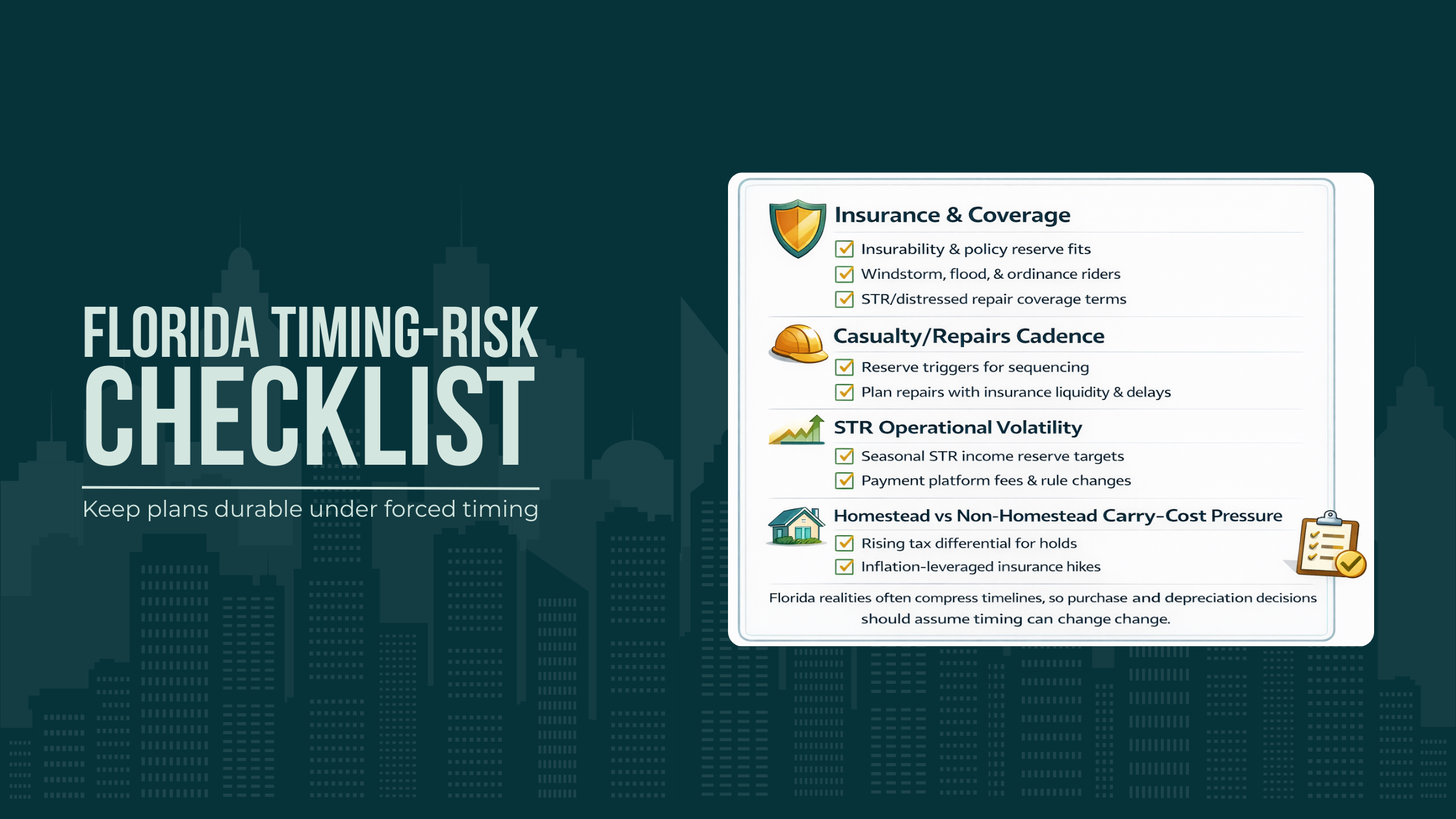
Florida realities often compress timelines, so purchase and depreciation decisions should assume timing can change.
Real estate concentration amplifies exit/recapture exposure
Florida investors often hold more real estate (and more types: STRs, long-term rentals, mixed-use). That concentration increases the odds of:
multiple dispositions in a short time window,
clustering gains into a single tax year,
accumulating depreciation history that creates a large §1250 stack at exit.
It also increases the odds that your “exit” is not fully elective. Insurance pricing, coverage availability, or casualty-related rebuilding decisions can compress timelines. When timelines compress, tax planning becomes sequencing under constraint—another reason to avoid asset purchase decisions that increase exit-year fragility.
Homestead vs non-homestead property tax realities affect holding decisions
While homestead is primarily a property-tax concept, the planning implication is behavioral and financial:
non-homestead carrying costs can rise faster,
which can shorten hold periods or force sale/refinance decisions,
which then interacts with the depreciation/unwind profile of the asset.
For HNW Florida taxpayers, the key is to treat carrying-cost volatility as a planning input. If a property is likely to be sold sooner because its carrying cost profile is unstable, your depreciation cadence should reflect that.
Insurance/casualty/climate risk changes timing, reserves, and exit planning
In Florida, forced timing is a real risk:
insurance premium changes,
coverage availability,
casualty events and repairs,
tenant disruption (especially with STR operations),
can all compress timelines.
A resilient tax plan includes:
liquidity and reserve design,
scenario planning for early sale,
sequencing rules that can be executed under stress.
Two Florida-specific execution points often matter:
Improvement cycles can be non-discretionary. Hardening projects, roof work, flood mitigation, and other insurance-driven improvements can shift large costs into specific years. If you treat those costs as “just another deduction,” you can accidentally create a year with large depreciation placements followed by a forced sale year where the unwind is concentrated.
STR operations add volatility and classification complexity. STR portfolios can swing between operational intensity and passive-like behavior depending on management approach and local conditions. That volatility can change NIIT exposure and loss usability over time, making set-and-forget asset purchase strategies more fragile.
A Florida planning nuance that shows up in real portfolios: when repairs and improvements cluster after a storm season (or after insurer-driven requirements), the tax profile of the property can change quickly. If you are also considering a sale or a refinance window, those timing collisions can be expensive. A coordinated plan explicitly sequences (a) improvement placement, (b) the probability of sale, and (c) liquidity reserves—so a post-improvement sale doesn’t inadvertently convert “cash-flow help” into a concentrated recapture stack.
We’ll review whether your entity and ownership structure preserves allocation flexibility and reduces the odds of an expensive, compressed exit-year stack.
Conclusion: the durable way to do asset purchase tax planning
Asset purchases don’t inherently increase tax exposure. Fragmented planning does.
The durable approach is to treat asset purchase tax planning as a coordinated system:
model the multi-year income stack (not just this year),
plan NIIT exposure as a core layer, not an afterthought,
pair depreciation strategy with an explicit unwind plan (sale/refi/hold scenarios),
align entity/ownership structure with flexibility and execution,
design the plan around operational reality—especially Florida’s real estate concentration and timing risks.
When those pieces are integrated, asset purchases can be a powerful part of long-term tax efficiency. When they are not, the “write-off” becomes a future tax concentration—often in the worst possible year.
A practical closing rule: we should be able to explain, in one sentence, why the deduction is being taken in this specific year and what the plan is for the year the basis reduction comes back. If we can’t, the plan is probably tactical, not strategic—and the odds of long-term tax leakage rise.
Bring one planned purchase or renovation and we’ll confirm the sequencing across tax years, including NIIT exposure and the recapture/unrecaptured §1250 implications at sale.
Frequently asked questions
How do we decide which year to place assets in service when income is volatile?
When income swings year to year, the best placement date is usually the year where the deduction reduces the most expensive “top layer” of your stack and doesn’t create a future exit-year concentration you can’t control. We typically compare at least two sequencing paths: (1) front-load deductions into a high ordinary-income year versus (2) spread placements to preserve flexibility for a future sale, refinance, or partner change. The decision often depends on whether the deductions will be usable (active vs passive constraints) and whether a likely disposition year would already be NIIT- and gain-heavy.
How do we avoid “stack collisions” when multiple transactions are possible across years?
Exit-year pileups happen when ordinary income, large gains, and recapture components land in the same tax year. The mitigation is less about any single tactic and more about choreography: we identify which events are truly controllable (renovation timing, placed-in-service dates, elective dispositions) and which are not (insurance-driven repairs, partner decisions, liquidity needs). Then we sequence controllables to create “cleaner” years for exits and “heavier” years for deductions. For Florida-heavy portfolios, we also plan for forced timing scenarios so the plan still works if the calendar gets compressed.
When does accelerated depreciation increase long-term tax cost even if we hold the property for years?
It may increase long-term cost when it shifts too much future gain into higher-tax character layers at exit—especially if the eventual sale year is already high-income or includes multiple dispositions. The issue isn’t that depreciation exists; it’s the composition of the unwind. Cost segregation can change how much gain is treated as recapture versus other categories, and basis reduction can make the sale-year stack more sensitive to NIIT layering. If the portfolio has a meaningful chance of an earlier-than-expected exit (insurance, casualty, capital needs), overly aggressive acceleration can turn deferral into expensive concentration.
How should we think about recapture and §1250 exposure if we’re not sure we’ll sell (or we might refinance instead)?
We treat recapture and §1250 exposure as a “latent stack” that becomes relevant whenever a sale happens—whether planned or forced. If refinance is the base case, we still model the sale scenario because refinances don’t erase depreciation history; they simply change the probability distribution of when a sale occurs. A durable plan usually includes two tracks: a hold/refinance track that uses accelerated depreciation only to the extent it improves long-run cash deployment, and a sale track that limits exit-year character concentration if timing shifts.
What entity or ownership choices most affect the long-term tax result of asset purchases?
The highest-impact choices are the ones that determine (1) how income and gain are characterized as they flow to owners, (2) whether allocations and control can adapt when facts change, and (3) whether participation status is supportable over time. In practice, the wrong structure isn’t “wrong” because of a single tax rate—it’s wrong because it removes options: you can’t sequence dispositions cleanly, you can’t align active vs passive outcomes with reality, or you can’t restructure without triggering friction or tax leakage. We look for structures that preserve optionality for partial exits and changing ownership.
How do passive-loss limitations change the sequencing value of asset purchases for high earners?
Passive limitations can turn a “good” deduction into a timing mismatch: the loss may be suspended and only become useful later, often in a year dominated by gains and recapture where the marginal benefit is smaller than expected. For sequencing, the key is not just how large the depreciation is, but whether it will actually reduce tax in the year you’re targeting. If the losses are likely to be suspended, we often prioritize purchases and placements that improve operational economics first and treat the tax benefit as secondary—then design a disposition strategy that uses released losses efficiently without creating an exit-year pileup.
What is the most Florida-specific risk that changes how we time purchases, improvements, and exits?
Florida’s no state income tax environment increases the importance of getting the federal character and sequencing right, but the bigger practical nuance is timing risk. Insurance pricing, coverage availability, and casualty-driven repair cycles can compress timelines and force major capex or dispositions. That means “we’ll just hold longer” is often not a complete plan. For STR-heavy portfolios, operational intensity can shift over time, changing classification and NIIT exposure. We plan with a forced-timing scenario so that improvements and depreciation choices don’t accidentally create a concentrated unwind in the first year you lose control of timing.
How do we handle “deduction decisions” when we also expect retirement transitions or changing work intensity?
Retirement transitions often create windows where the income stack is structurally different—sometimes lower, sometimes constrained by other income streams. Asset purchases and depreciation choices should preserve the ability to use those windows for clean exits or strategic repositioning. If your plan assumes you’ll sell in a lower-income phase, then front-loading depreciation that increases future exit-year character concentration may work against you if the sale slips into a higher-income year. We typically coordinate purchase timing, likely disposition timing, and ownership/participation realities so the plan remains viable as work intensity and cash-flow priorities shift.