2026 Long-Term Capital Gains Tax Brackets: A Strategic Framework for High-Income Florida Taxpayers
A coordinated framework keeps exit-year character and NIIT from turning one sale into a multi-layer rate surprise.
High-income Florida taxpayers tend to underestimate how “capital gains planning” quietly becomes federal rate engineering. With no Florida state income tax, you don’t have a state layer to optimize or cushion—so the quality of your federal sequencing decisions shows up directly in after-tax wealth: how gains stack on top of ordinary income, whether NIIT layers on, how real estate depreciation unwinds at exit, and how entity structure and passive/active classification constrain your options.
For sophisticated investors and business owners, the real question isn’t “what’s the rate?” It’s: how do we design a multi-year income pattern—ordinary income, investment income, and real estate exits—so long-term capital gains land in the most efficient layers while preserving flexibility if the plan needs to change?
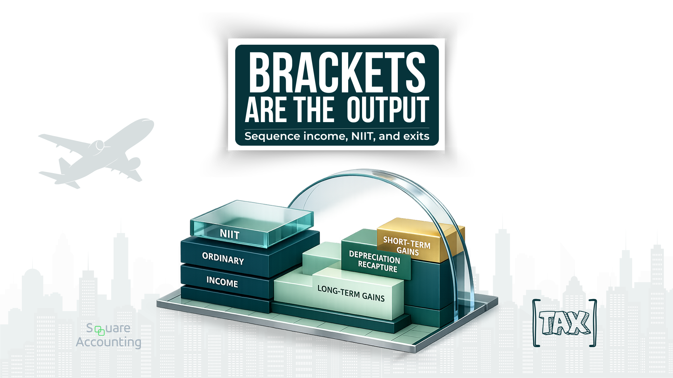
The 2026 long-term capital gains tax brackets are only one layer of the decision. The real outcome comes from how ordinary income stacks first, whether NIIT overlays the gain, and how real estate sale character behaves at exit.
In this article we use the 2026 long-term capital gains tax brackets as the organizing framework, then stress-test that framework against real-world Florida profiles: business income variability, real estate concentration, short-term rental cash flow swings, and insurance/casualty timing risk. The objective is not a one-year “savings” story; it’s a durable sequencing logic that still works when an exit happens earlier than expected.
Key takeaways
Capital gains rates are stacked, not isolated. Your long-term capital gains bracket is determined by taxable income, after ordinary income consumes lower layers first—so timing and income smoothing can matter more than the asset itself.
NIIT is frequently the true marginal rate for high earners. For many Florida taxpayers, the difference between a “15% gain” and a materially higher effective rate is the 3.8% NIIT layer and how your income is classified and paced across years.
Real estate exits produce multiple tax “buckets” inside one sale. Depreciation-related gain components and unrecaptured §1250 gain can raise the effective marginal rate on part of the disposition, which makes holding period strategy and depreciation pacing multi-year decisions.
Cost segregation is best treated as an income-shaping tool, not a trophy deduction. Accelerating depreciation can improve near-term cash flow and reduce current taxable income, but it also changes the character mix and NIIT exposure at exit—especially if the holding period shortens.
Entity and ownership structure determine which levers you actually have. Allocation flexibility, installment pacing, charitable techniques, and who bears NIIT can all hinge on how the gain flows through ownership and activities.
Florida’s environment amplifies concentration and timing risk. Heavy real estate exposure plus insurance/casualty volatility means exit optionality and liquidity reserves are part of tax strategy, not separate “financial planning” topics.
We’ll map a multi-year corridor so gains, NIIT exposure, and exit-year depreciation unwind don’t stack unpredictably.
The 2026 long-term capital gains rate structure (what the brackets actually mean)
For most long-term capital gains (assets held more than one year) and qualified dividends, the federal rate structure uses three preferential layers: 0%, 15%, and 20%. The practical trap is assuming those layers apply “to the transaction.” They don’t. They apply to the portion of your net long-term gain and qualified dividends that falls into each layer after ordinary income has already taken its place in the stack.
Two technical points drive planning outcomes:
These thresholds are based on taxable income, not “capital gains income.” Ordinary income fills lower layers first; long-term gains then stack on top.
Not all gain in a long-term real estate sale is treated as standard long-term capital gain. Depreciation-related components can be pulled into separate categories with different maximum rates, changing the effective marginal rate even if the sale is long-term.
2026 long-term capital gains tax brackets (by filing status)
Below are the taxable-income thresholds for the 0% and 15% long-term capital gains layers in 2026. Amounts above the 15% ceiling generally fall into the 20% long-term capital gains layer.
| Filing status | 0% LTCG up to | 15% LTCG up to | 20% LTCG above |
|---|---|---|---|
| Married filing jointly / Surviving spouse | $98,900 | $613,700 | $613,700 |
| Married filing separately | $49,450 | $306,850 | $306,850 |
| Head of household | $66,200 | $579,600 | $579,600 |
| Single (all other individuals) | $49,450 | $545,500 | $545,500 |
A strategic reminder: these are brackets for net long-term capital gain and qualified dividends, not a promise that your next sale “qualifies” for a given rate. The rate your gain actually sees is the rate that remains after your ordinary income, deductions, and other items have occupied lower layers.
Income stacking in practice: why high earners rarely “choose” the 15% bracket
Most high-income Florida business owners and professionals already carry substantial ordinary income (W-2, K-1, self-employment, guaranteed payments, or other earned income). Because ordinary income stacks first, it often consumes the entire 0% capital gains layer and part of the 15% layer before the first dollar of long-term gain is taxed.
For high earners, the key lever is rarely the asset—it’s the year. A corridor approach separates ordinary-income-heavy years from capital-event-heavy years so bracket capacity isn’t consumed before the gain arrives.

Sequencing across years protects bracket capacity and reduces compounding effects when timelines compress.
This is why a “capital gains strategy” that ignores ordinary income variability is incomplete. In practice, the planning problem is: what else is happening in the same year?
Examples that frequently change the capital gains outcome:
A business owner takes a larger distribution in an otherwise “exit year,” pushing taxable income above the 15% ceiling and converting part of the gain into the 20% layer.
Partnership K-1 income spikes due to a one-time event, crowding out the 15% layer for portfolio gains and making loss strategy and charitable technique selection materially more valuable in that year.
A real estate investor sells one property in a year that also includes a concentrated portfolio rebalance—turning what looked like a “15% sale” into a multi-layer event with NIIT stacking on top.
The planning implication
The lever is rarely “sell vs. don’t sell.” The lever is when you recognize gain relative to:
(1) high ordinary-income years, (2) unusually low ordinary-income years, and (3) years where your deduction profile is structurally different.
We find it useful to build an “income corridor” across 3–5 years. In corridor years, we avoid unnecessary ordinary-income spikes and avoid stacking multiple capital events together unless there is a compelling business reason. Then we choose the year in which a planned long-term gain is recognized, and we ensure that year has the capacity to absorb the gain in the intended layers.
For HNW Florida taxpayers, this is often the point where tax planning stops being about isolated tactics and becomes about multi-year governance: deciding which years are “income heavy,” which years are “capital gains heavy,” and which years are designed to rebuild optionality.
NIIT layering: the difference between a 15% gain and a 23.8% gain
The Net Investment Income Tax (NIIT) is a 3.8% surtax that applies to certain investment income when modified adjusted gross income exceeds threshold amounts. Importantly for multi-year planning, the IRS notes the NIIT thresholds are not indexed for inflation. That means more high-earning households are pulled into NIIT over time even if their “real” income hasn’t changed.
NIIT is computed on the lesser of (a) net investment income or (b) the excess of MAGI over the threshold. This creates two different planning environments:
Partial NIIT years: MAGI exceeds the threshold by a modest amount, so only part of net investment income is exposed.
Full NIIT years: MAGI exceeds the threshold by a wide margin, so (practically) all net investment income is exposed.
NIIT thresholds (and why they matter so often in Florida)
NIIT generally applies when MAGI exceeds: $200,000 (single/head of household), $250,000 (married filing jointly), or $125,000 (married filing separately). These amounts sit directly in the income ranges where many Florida entrepreneurs and investors operate—especially in years that include a real estate disposition, a liquidity event, or a concentrated portfolio rebalance.
For Florida taxpayers, NIIT tends to be the decisive layer because there is no state tax offset. With no Florida income tax, “federal + NIIT” often becomes the whole marginal story in an exit year.
Strategic takeaway
For high earners, NIIT frequently turns the practical question into: can we structure income and activities so the gain is not treated as net investment income—or so MAGI doesn’t spike in the exit year?
There are two distinct levers:
Classification: Whether an item is net investment income depends on facts and structure. NIIT is not just a portfolio issue; passive rents and certain gain categories typically remain in the NIIT base, while income tied to an active trade or business may have different treatment depending on the facts.
Pacing: NIIT is MAGI-triggered. Even if the gain is net investment income, spreading recognition over more than one year can reduce the portion exposed in any single year—especially in partial NIIT years.
In an exit year, we also treat estimated tax governance as part of the strategy. It doesn’t change the rate, but it prevents forced liquidity decisions later. If you want the option to control recognition timing, you need the cash management to support that option.
We’ll identify where NIIT is driving your marginal rate and design sequencing that avoids unnecessary MAGI spikes in exit years.
Exit planning for real estate: depreciation recapture, unrecaptured §1250 gain, and unwind scenarios
Real estate exits are where capital gains planning most often breaks down, because a single sale can create multiple tax characters:
portions taxed at preferential long-term capital gains rates,
portions taxed under special capital gain categories (including unrecaptured §1250 gain for depreciable real property), and
potential NIIT layering depending on your facts.
The IRS explicitly notes that the portion of any unrecaptured section 1250 gain from selling section 1250 real property is taxed at a maximum 25% rate, separate from the general 0%/15%/20% structure.

Exit planning improves when we treat the sale as a character waterfall and manage what else stacks into the same year.
We’ll pressure-test your sale-year character mix, including unrecaptured §1250 gain and bracket stacking, across multiple timing paths.
Why this changes the multi-year plan
Real estate is unique because you often take depreciation benefits over years, then face a character shift at sale. If you used cost segregation to accelerate depreciation, you improved early-year cash flow and reduced taxable income, but you also changed the character mix at exit. The exit year becomes a “rate compression” year: higher MAGI, more NIIT exposure, and more gain sitting in higher-rate buckets.
That creates a second-order effect many high earners miss: the best exit-year plan starts years before the sale. The pre-sale period is when you decide how aggressively to accelerate depreciation, how to manage passive loss build-up, and whether to structure ownership and participation so the NIIT outcome at sale is known and controlled.
A long-term hold doesn’t guarantee a single long-term capital gain rate at sale. This matrix highlights when depreciation history and NIIT layering are likely to drive marginal cost—and which levers matter before you list.
Unwind scenarios that deserve explicit modeling
High-income Florida real estate investors commonly face unwind patterns where tax strategy meets reality:
Refinance-to-hold becomes sell earlier than expected due to insurance premium shocks, HOA changes, capex surprises, partnership friction, or STR cash flow volatility.
A 1031 intent becomes portfolio simplification because concentration risk becomes unacceptable after underwriting assumptions change.
A passive-to-active shift occurs late, but the exit-year classification and prior-year grouping decisions determine what losses are usable at sale.
A partnership member wants out, forcing a partial disposition at a time that is not tax-optimal for the group.
We treat these as normal, not exceptional. The planning objective is to build an exit plan that still works if the sale happens in Year 2 instead of Year 5, and that includes a decision tree for “sell vs hold vs exchange vs partial exit” under different market and insurance conditions.
A practical tool here is to pre-model your sale as a tax character waterfall: depreciation-related components (including unrecaptured §1250 gain), residual long-term capital gain, then overlay NIIT. The point is not to compute the penny; it’s to identify which component is the true driver of marginal rate and which levers actually affect it.
Cost segregation as a planning tool, not a tactic
Cost segregation is often discussed as “front-loading deductions.” For sophisticated taxpayers, the better framing is: cost segregation changes the timing and character of taxable income—and therefore changes which layers your future capital gains land in.
When cost segregation strengthens the capital gains plan
Cost segregation can be strategically strong when:
You can reasonably defend the holding period based on economics and risk (not optimism).
You can absorb depreciation without wasting losses (or creating a passive-loss inventory that cannot be used in your expected exit window).
You have an exit-year plan that anticipates character effects, NIIT exposure, and the possibility of an earlier sale.
A particularly effective use case is when cost segregation is paired with a clear “income corridor” plan: you intentionally lower taxable income in Year 1 and Year 2 to preserve cash, then in the planned exit year you avoid stacking additional ordinary-income spikes and you manage other capital events so the sale is absorbed in the intended layers.
Where it commonly backfires
It backfires when:
Accelerated depreciation reduces taxable income today but increases NIIT exposure later by raising MAGI in the exit year when the unwind happens at scale.
Passive loss limitations make the “benefit” paper-only for years, while the exit still triggers taxable gain and possible NIIT.
The plan assumes a holding period that Florida’s insurance and capex realities don’t support; a forced sale compresses the entire strategy into a single year.
Our bias is not “use less cost segregation.” Our bias is to apply it as part of an integrated exit strategy. If the depreciation profile is not coordinated with holding period realism and the exit-year tax character, cost segregation becomes a volatility amplifier.
Entity and ownership structure: how the gain flows determines your options
Entity structure determines how gains flow, how losses are trapped or released, and which owners face NIIT exposure. For multi-entity Florida taxpayers—common among real estate investors and business owners—structure is frequently the difference between a controlled, paced recognition event and an uncontrolled spike.
Partnership vs. S corporation vs. disregarded entity: the planning constraints
At a high level:
Partnerships/LLCs taxed as partnerships can offer allocation flexibility, but that flexibility comes with governance requirements: allocations must be defensible, consistent with the operating agreement, and economically grounded.
S corporations are more rigid on allocations and compensation mechanics. That rigidity can matter because compensation and pass-through income affect the ordinary income base that uses up favorable capital gain layers.
Disregarded entities keep planning at the individual level, which can simplify stacking analysis but can limit structural levers in multi-owner situations.
Two advanced planning implications are often overlooked:
Flexibility at the owner level can be more valuable than entity-level optimization. A partnership structure that allows owners to handle buyouts or partial exits without forcing everyone into the same year can preserve bracket capacity and reduce NIIT compression.
Ownership architecture affects the feasibility of pacing mechanisms. Installment structures, partial redemptions, and charitable techniques are often constrained by how title is held and how debt is structured.
If your current entity structure was chosen for acquisition convenience, it may be misaligned with disposition reality. In Florida, that misalignment is common because investors assemble portfolios quickly, then later realize a simplified structure created inflexible exits.
We’ll review how your entity and ownership flow affects pacing options and NIIT outcomes when the disposition year arrives.
Active vs. passive treatment: why this becomes binding at exit
Sophisticated investors often treat active vs passive rules as an annual loss-usage issue. In reality, the sale year is where classification becomes binding because it determines whether losses can offset the income you actually have and whether NIIT applies to the gain.
There are two recurring failure modes:
Passive losses accumulate for years while cash flow remains strong, but the investor assumes those losses will “handle” the exit. Then the exit-year income includes components that don’t pair efficiently with the passive-loss pool, and NIIT may still apply to significant portions.
The investor’s participation profile changes over time (for example, moving from passive to more active involvement), but grouping decisions and activity design were never coordinated with the exit. When a disposition occurs, the expected release of losses is smaller or occurs under different rules than assumed.
For a high-income household, this is not academic. The sale-year tax outcome can swing materially based on whether the activity is treated as passive, and how suspended losses are released relative to the gain character buckets.
We approach this by treating activity design as part of the exit plan: we map which activities generate passive income, which generate passive losses, and which are expected to generate disposition events. Then we ensure the plan does not rely on “paper offsets” that only work under one narrow fact pattern.
Cash flow vs. long-term tax efficiency: where “tax savings” quietly becomes risk
High-income Florida taxpayers often face a real trade-off: front-load deductions to improve near-term cash flow, or preserve basis and flexibility so the exit year is manageable. The problem is that many strategies look optimal only under stable assumptions: stable insurance costs, stable occupancy, stable capex, stable financing.
Florida is not a stable-assumption environment for real estate. Insurance repricing, storm-related repairs, and capex surprises create timing risk that can force dispositions or refinancing decisions on a schedule that is not tax-optimal.
Two second-order effects deserve explicit treatment:
Liquidity stress turns tax planning into forced selling. If you don’t have reserves for premiums, deductibles, and repairs, you lose the ability to choose the year of recognition. That is a bracket problem, not just a cash problem.
Cash flow optimization can raise exit-year friction. Maximizing near-term depreciation benefits without a matching exit plan can create a larger portion of gain in higher-rate buckets later.
The strategic discipline is to prefer strategies that preserve optionality under timing shocks. A plan that wins only if everything goes right is a bet, not a tax strategy.
Retirement, pensions, and RMD coordination: capital gains planning doesn’t live in a silo
For many high earners, the best capital gains year is the year you also reduce earned income intentionally, coordinate retirement plan contributions or distribution timing, and avoid stacking gains on top of unusually high ordinary income.
The trap is assuming retirement planning and capital gains planning are separate workstreams. In reality:
Ordinary income levels determine how much of the 0%/15% layers are already consumed.
Retirement distributions can crowd out favorable capital gain layers in later years.
Pension contributions can be used as pacing tools, but only when coordinated with compensation structure and cash flow.
Two planning patterns are especially common in Florida HNW households:
The “RMD crowd-out” pattern: investors defer coordination for years, then RMDs and other fixed-income streams arrive at the same time as planned asset sales. The result is compressed bracket capacity and higher NIIT exposure in the years when the household wants liquidity most.
The “retirement corridor” opportunity: if a household anticipates a drop in earned income (sale of a practice, scaled-back business operations, major restructuring), there may be a limited window where taxable income capacity is lower. That can be a strategic time to recognize gains intentionally—provided it is coordinated with real estate exit mechanics and portfolio needs.
The overarching principle is that retirement and capital gains planning share the same scarce resource: bracket capacity. When we plan them together, the plan tends to be more durable.
Asset-based planning vs. deduction-first planning: the framework high earners actually need
A deduction-first approach asks: what can we write off this year?
An asset-based approach asks:
Which assets are likely exits in the next 3–7 years?
Which exits will generate depreciation unwind complexity (including unrecaptured §1250 gain)?
Which holdings are vulnerable to Florida-specific timing shocks (insurance/casualty, STR variability, capex)?
Which entity structures preserve the ability to pace recognition or shift the burden across owners?
In other words: we plan around exits and capital events first, then use deductions and depreciation as tools to shape the path without sacrificing resilience.
This perspective also clarifies what “good” looks like: not the lowest tax this year, but a coherent, repeatable system for deciding which events happen in which year and how the tax character will behave when the plan meets reality.
Putting it together: a 3-year sequencing example (no gimmicks, just mechanics)
Consider a Florida taxpayer with consistently high ordinary income from a business, a real estate portfolio with one property likely to be sold within 24–36 months, and periodic investment gains from a brokerage portfolio.
A strategic sequencing approach might look like this.
Year 1: Create flexibility, not noise
Stabilize ordinary income where possible (compensation policy, distribution timing, discretionary business deductions).
Avoid triggering large capital gains unless there is a compelling asset reason.
Use depreciation strategies only to the extent they create usable value, not trapped passive losses.
Build liquidity reserves explicitly for Florida insurance/casualty volatility so recognition timing remains a choice.
Year 2: Build the “exit corridor”
If a sale is likely, avoid stacking additional gain sources such as major portfolio rebalancing or optional business distributions.
Evaluate pacing options early: partial exits, installment features where viable, charitable tools where aligned, and the governance required for multi-owner properties.
Confirm the activity classification and loss posture that will govern the sale year, not just the current year.
Year 3: Execute the exit with rate control
Manage taxable income layers so the gain lands as efficiently as possible within the long-term capital gains brackets.
Model depreciation-related components so you’re not surprised by higher-rate buckets at closing.
Confirm whether NIIT applies and whether pacing or classification levers exist in your facts.
Treat the sale year as a coordination year: avoid unrelated capital events that don’t belong in the same stack.
The point is not that every investor should follow this timeline. The point is that the sale year should be designed, and the design work begins before the listing agreement—not at closing.
Correcting common misuse and oversights
This is where we see sophisticated taxpayers—people with good CPAs and solid wealth advisors—still lose efficiency.
1) Treating long-term gains as a single rate
Many plans assume “it’s long-term, so it’s 15%.” In reality: ordinary income stacking determines which layers are available; NIIT can add 3.8%; and real estate depreciation-related components can create separate higher-rate buckets.
2) Over-optimizing the current year without modeling the exit year
A strategy that improves Year 1 but worsens Year 3 isn’t automatically wrong, but it must be intentional. If an exit is likely within a few years, you need an exit-year model, not just a tax return optimization.
3) Letting entity structure be “historical” instead of strategic
Entities that were fine at acquisition can become suboptimal at disposition—especially if ownership, participation, financing, or risk profile changes. Structure determines maneuvering room when timing shifts.
4) Ignoring NIIT until it appears
NIIT is not a rounding error in high-income years, especially in Florida where there is no state layer. If a plan doesn’t explicitly address NIIT, it’s incomplete for many HNW households.
5) Assuming holding period certainty in a Florida risk environment
Insurance repricing, casualty exposure, and capex volatility create real pressure on holding periods. If your tax plan requires a long holding period to “work,” it should include a credible contingency path for an earlier sale.
We’ll coordinate ordinary income, long-term gains, and real estate timing so bracket capacity is protected and passive/active constraints don’t bind at exit.
Florida-specific planning considerations that change the analysis
Florida’s “no state income tax” environment is often discussed as a benefit—and it is—but it also shifts the full burden of optimization onto federal planning. There’s no state bracket engineering to offset mis-sequencing at the federal level.
Florida’s no state income tax environment concentrates the outcome in federal stacking and NIIT. These checklist items are common reasons holding periods compress—so we build reserve policy and an exit decision tree into the plan.

In Florida, timing shocks often drive exits—reserves and decision rules keep sequencing intact when conditions change.
1) Federal planning carries more weight without a state layer
In high-tax states, capital gains outcomes are influenced by state sourcing and state rate structure. In Florida, the outcome is dominated by federal stacking, NIIT exposure, depreciation unwind character, and entity/participation classification. That concentrates the value of getting federal sequencing right.
2) Florida real estate concentration increases exit/recapture exposure
Many Florida high earners are overweight real estate, often with short-term rental activity. That means more depreciation strategies in play, more likelihood of exit-year character complexity, and more need for multi-year pacing. In a concentrated portfolio, one sale can shift the household’s entire tax profile for the year.
3) Homestead vs. non-homestead property tax realities affect hold/sell choices
We don’t treat property tax as a local law seminar, but planning-wise the distinction matters because it influences carry cost, liquidity needs, and the likelihood of early sale. If a property’s non-homestead carrying cost rises materially, the decision to hold becomes a capital allocation decision—and that decision determines whether you face an earlier-than-planned gain recognition event.
4) Insurance/casualty/climate risk changes reserve policy and timing risk
Florida’s insurance and casualty reality changes the “time optionality” of real estate. A purely tax-optimized holding plan can collapse if reserves are insufficient when premiums spike or major repairs are required. Better planning treats liquidity reserves, capex timing, and exit optionality as part of the tax strategy because they determine whether you can choose when you recognize gain.
Two practical planning add-ons that often improve durability:
Pre-commit to an exit decision tree triggered by objective thresholds (coverage cost as a percentage of NOI, deductible levels, recurring capex, or occupancy volatility). This reduces the odds that tax-inefficient timing decisions are made under stress.
Align insurance/casualty reserve policy with tax pacing. If the sale year becomes likely, reserves can be adjusted to avoid forced liquidity events that stack on top of the disposition.
The goal is not to predict the next storm season. The goal is to build a plan that remains coherent under volatility.
Do qualified dividends use the same 2026 brackets as long-term capital gains?
Generally, qualified dividends are taxed using the same preferential rate layers and the same taxable-income thresholds as long-term capital gains. Strategically, this means dividend-heavy portfolios should be modeled alongside sale gains and business income, because qualified dividend income consumes the same bracket capacity that long-term capital gains would otherwise use.
If we’re in Florida, is capital gains planning less important because there’s no state tax?
Usually the opposite. Without a state layer, your outcome is dominated by federal stacking and NIIT. That makes federal sequencing decisions more consequential, not less.
Why do real estate exits feel “more expensive” than expected even when held long-term?
Because the sale can contain multiple tax characters: standard long-term capital gain layers, depreciation-related gain components including unrecaptured §1250 gain (taxed at a higher maximum rate), and potential NIIT on top. If you model a sale as “sale price minus basis times 15%,” you’re not modeling the real tax profile.
Conclusion: use the 2026 brackets as a framework, not a target
The 2026 long-term capital gains tax brackets are the visible part of the system. For high-income Florida taxpayers, the planning outcome is driven by interactions: ordinary income stacking determines which layers are available; NIIT often sets the true marginal rate; and real estate exits introduce character complexity that must be designed for years before the listing.
A durable plan is coordinated across tax years: income pacing, entity and ownership architecture, depreciation strategy with an explicit exit model, and contingency paths for the timing shocks that are common in Florida’s real estate-heavy environment. The goal isn’t to pay the lowest rate this year. The goal is to build a multi-year system where capital events land in efficient layers without sacrificing flexibility.
We can walk through an exit-year sequencing review focused on bracket stacking, depreciation unwind dynamics, and the cash flow vs. long-term efficiency trade-off.
Frequently asked Questions
How do we decide whether to realize gains in the same year as high ordinary income?
If ordinary income is already consuming most of your bracket capacity, layering long-term gains on top can push more of the gain into less favorable layers and increase the likelihood that NIIT becomes fully binding. The strategic question is whether the gain is optional (portfolio repositioning, discretionary sale) or driven by asset risk (tenant, insurance, capex, partnership dynamics). When it’s optional, we often prefer separating “ordinary-income-heavy” years from “capital-event-heavy” years, so you’re not paying for two stacks at once. When it’s not optional, the focus shifts to pacing and character management.
What’s a practical way to sequence multiple capital events across 2–3 years without losing flexibility?
We start by ranking capital events by reversibility and risk: events you can delay (rebalancing, discretionary sales) versus events that may force timing (refinance maturity, insurance repricing, partnership buyouts). Then we build a corridor: one year designed to absorb a major exit, adjacent years kept “clean” by avoiding avoidable gains and unusual ordinary-income spikes. This approach isn’t about perfect forecasting; it’s about protecting bracket capacity and reducing compounding effects when reality compresses timelines.
When should we model a real estate sale as more than “long-term capital gain”?
Often when the property has meaningful depreciation history, cost segregation activity, or a long hold with multiple improvement cycles. In those cases, the sale tends to include different tax characters—some of which can behave differently than standard long-term capital gains—and the effective marginal rate becomes a blend driven by the character waterfall. Modeling this early matters because it influences pre-sale decisions: whether to accelerate depreciation, whether to clean up suspended loss positions, and whether to avoid stacking other capital events into the same year.
How do depreciation strategies change the exit-year outcome in ways investors underestimate?
Depreciation acceleration can improve near-term cash flow, but it also shifts how much gain is tied to depreciation-related components when you sell. That can turn an exit year into a higher-friction year—more income character complexity, more MAGI pressure, and a greater chance that NIIT becomes fully binding. The key is not “avoid depreciation,” but to pair depreciation choices with an exit design: realistic holding period assumptions, a pacing plan if the timeline shortens, and a clear view of which components are driving marginal tax cost.
What should we do differently if an early sale becomes likely due to insurance, capex, or STR volatility?
An early-sale likelihood changes the priority from “optimize annual taxable income” to “protect the disposition year.” Practically, that can mean reducing avoidable income spikes, avoiding discretionary capital gains, and tightening liquidity governance so you don’t force a sale or a portfolio liquidation under stress. It also means revisiting whether depreciation pacing still fits the new timeline and whether ownership or partnership dynamics could force timing. Florida-specific risks often compress timelines; the plan needs a contingency path that’s still coherent if the hold shortens.
How does entity and ownership structure influence our ability to control the tax outcome of an exit?
Structure determines which levers exist in the year the gain is recognized: how income flows to owners, what flexibility exists for pacing, and whether one owner’s timing needs force everyone into the same year. In multi-owner real estate, this can be the difference between a managed disposition and an uncontrolled spike. We also look at whether the structure aligns with how the asset is actually operated, because classification and activity design can influence whether NIIT becomes the dominant marginal layer. If structure was chosen for acquisition speed, it may not fit disposition complexity.
Why does Florida’s “no state income tax” environment make federal sequencing more important, not less?
Without a state income tax layer, more of the outcome is concentrated in federal stacking and NIIT layering. That concentration makes “bracket capacity” a more valuable resource and makes the cost of poor timing more visible. Florida realities also affect timing: property tax carry-cost differences, short-term rental revenue variability, and insurance/casualty risk can push investors into earlier-than-planned decisions. The tax plan can’t assume stable holding periods; it needs reserves, an exit decision tree, and sequencing discipline so timing shocks don’t create compounded tax friction.
How do we evaluate whether a “clean year” for gains is actually clean for a high-income household?
A year can look clean on the capital gains side but still be compromised by ordinary-income events, K-1 volatility, or retirement distribution patterns that crowd out bracket capacity. We test “clean” by looking at what’s likely to be non-discretionary: business income swings, planned distributions, debt-driven transactions, and any events that can’t easily move across years. Then we evaluate whether the capital event you want to place there will trigger second-order effects—particularly NIIT becoming fully binding. A clean year is one where the stack is intentionally shaped, not merely “quiet.”